Author:baiyucraft
BLog: baiyucraft’s Home
Paper: Single Shot MultiBox Detector
gihub: MySomeNet
一、算法重现 1.SSD简介 首先,我们得知道什么是SSD:
SSD算法是一种one-stage 单阶段的目标检测算法,基于回归思想和Anchor机制,采用多尺度特征金字塔检测方式进行预测。
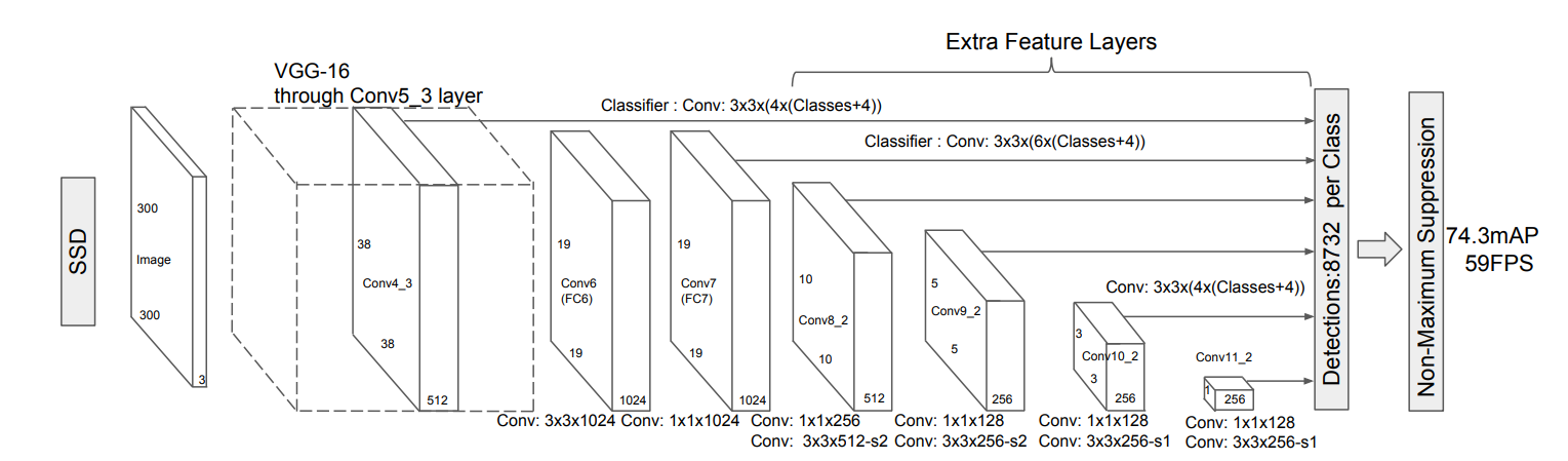
以下是SSD算法的模型结构图:
实际上在看到这个结构图的时候,只能知道该模型做的一系列卷积操作以及输出特征图的大小,接下来让我们以输入图像大小为300*300的SSD300 为例,分模块讲述整个SSD网络。
2.网络结构
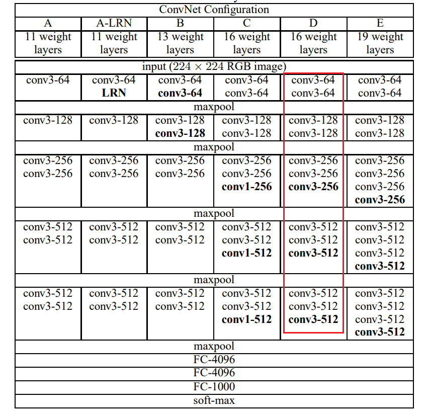
在SSD论文中使用的主干网络是如上图所示的VGG-16网络,取了VGG-16中的前五个卷积块,抛弃了后两个大的全连接层,具体实现如下:
1
2
3
4
5
6
7
8
9
10
conv_arch = [(2 , 64 ), (2 , 128 ), (3 , 256 ), (3 , 512 ), (3 , 512 )]def vgg_block (num_convs, in_channels, out_channels ):for _ in range (num_convs):3 , padding=1 ))True ))2 , stride=2 , ceil_mode=True ))return nn.Sequential(*layers)
1 2 3 4 5 6 7 8 9 10 11 12 13 14 15 16 17 18 19 20 21 22 23 24 25 26 27 28 29 30 31 32 33 34 35 36 37 38 39 40 41 42 def get_vgg_layer ():3 for i, (num_convs, out_channels) in enumerate (conv_arch):f'conv{i + 1 } _3' , vgg_block(num_convs, in_channels, out_channels))1 ][-1 ] = nn.MaxPool2d(kernel_size=3 , stride=1 , padding=1 )512 , 1024 , kernel_size=3 , padding=6 , dilation=6 ), nn.ReLU(inplace=True ))1024 , 1024 , kernel_size=1 ), nn.ReLU(inplace=True ))'conv6' , conv6)'conv7' , conv7)1 ][-2 ].out_channels256 , kernel_size=1 , stride=1 ),True ),256 , 512 , kernel_size=3 , stride=2 , padding=1 ),True ))512 , 128 , kernel_size=1 , stride=1 ),True ),128 , 256 , kernel_size=3 , stride=2 , padding=1 ),True ))256 , 128 , kernel_size=1 , stride=1 ),True ),128 , 256 , kernel_size=3 , stride=1 ),True ))256 , 128 , kernel_size=1 , stride=1 ),True ),128 , 256 , kernel_size=3 , stride=1 ),True ))'conv8_2' , conv8_2)'conv9_2' , conv9_2)'conv10_2' , conv10_2)'conv11_2' , conv11_2)return layers
在代码实现中可以看出,SSD模型在第5个卷积块后更改了池化的参数,并在第6个卷积的时候采用的是空洞率为6的空洞卷积,通过第六层的空洞卷积保持相较于VGG网络的感受野不变,在两个卷积后,又增加了四个卷积块 conv8_2、conv9_2、conv10_2、conv11_2,这四个卷积块所输出的都是之后要用到的特征图。
3. 针对特征图的先验框的生成 由SSD网络的结构图可知,整个SSD300的网络分别生成了如下表所示的6张不同尺度的特征图:
层 channels h*w conv4_3 在池化前的输出 512 38*38 conv7 的输出 1024 19*19 conv8 的输出 512 10*10 conv9 的输出 256 5*5 conv10 的输出 256 3*3 conv11 的输出 256 1*1
在SSD网络中。先针对每张特征图,针对每个像素,以每个像素为中心生成不同尺度和高宽比的先验框,具体生成的参数如下表所示:
特征图 宽高比 尺度范围(相对于图比例大小) 先验框个数/像素 C1 1、1/2、2 0.1 ~ 0.14 4 C2 1、1/2、2、1/3、3 0.2 ~ 0.272 6 C3 1、1/2、2、1/3、3 0.37 ~ 0.447 6 C4 1、1/2、2、1/3、3 0.54 ~ 0.619 6 C5 1、1/2、2 0.71 ~ 0.79 4 C6 1、1/2、2 0.88 ~ 0.961 4
其中以C1为例,宽高比为1的框分别以0.1和0.14的尺度范围生成,宽高比为1/2和2的,仅以0.1的尺度范围生成,所以每个像素点总共生成4个框。
综上,总共生成了 ∑ i = 1 6 C i ( h ) ∗ C i ( w ) ∗ C i ( n u m ) \sum_{i=1}^{6}{ C_i(h) * C_i (w) * C_i (num) } ∑ i = 1 6 C i ( h ) ∗ C i ( w ) ∗ C i ( n u m ) 8732个先验框,具体代码如下:
1
2
3
4
5
6
7
8
9
10
11
12
13
14
15
16
17
18
19
20
21
22
23
class PriorBox (object ):""" Args: feature_maps: 输入的特征图的大小 cfg: 一些参数 """ def __init__ (self, feature_maps, cfg ):super (PriorBox, self).__init__()'sizes' ]'ratios' ]'variance' ]def forward (self ):for i, f in enumerate (self.feature_maps)])max =1 , min =0 )return output
其中每个特征图的先验框生成具体如下:
1
2
3
4
5
6
7
8
9
10
11
12
13
14
15
16
17
18
19
20
21
22
23
24
25
26
27
def multibox_prior (data, sizes, ratios ):"""生成以每个像素为中心具有不同形状的锚框。""" 0 ], data[1 ]len (sizes), len (ratios)0.5 , 0.5 1 ), shift_x.reshape(-1 )for cx, cy in zip (shift_x, shift_y):0 ], sizes[0 ]]1 ], sizes[1 ]]for r in ratios:0 ] * sqrt(r), sizes[0 ] / sqrt(r)]0 ] / sqrt(r), sizes[0 ] * sqrt(r)]1 , 4 )return output
4.先验框的回归预测和分类预测 这一部分的具体参数可以从SSD模型结构图中看出,以C1为例,经过的是3×3的卷积核,得到通道数为 $ 4 × (4 + num_{classes})$ 的数据,第一个 4 4 4 4 4 4
b c x = p c x + l o c x ∗ p w ∗ v b c y = p c y + l o c y ∗ p h ∗ v b w = p w ∗ e l o c w ∗ v b h = p h ∗ e l o c h ∗ v b_{cx} = p_{cx} + loc_x * p_w * v \\ b_{cy} = p_{cy} + loc_y * p_h * v \\ b_w = p_w * e^{loc_w * v} \\ b_h = p_h * e^{loc_h * v} \\ b c x = p c x + l o c x ∗ p w ∗ v b cy = p cy + l o c y ∗ p h ∗ v b w = p w ∗ e l o c w ∗ v b h = p h ∗ e l o c h ∗ v
其中 b b b p p p l o c loc l oc c x 、 c y 、 w 、 h cx、cy、w、h c x 、 cy 、 w 、 h c_box 。
在具体实现中,将对框的回归预测和分类预测分成两个卷积层对同一个特征图计算完成,具体代码如下:
1
2
3
4
5
6
7
8
9
10
11
12
13
14
15
16
17
18
19
20
21
22
23
24
25
26
27
28
29
30
31
32
33
34
35
36
37
def get_multibox (layers, num_classes ):"""定义预测的卷积层""" 38 , 38 ), (19 , 19 ), (10 , 10 ), (5 , 5 ), (3 , 3 ), (1 , 1 )]3 ][4 ].out_channels'conv4_3_loc' , nn.Conv2d(in_channels, 4 * 4 , kernel_size=3 , padding=1 ))'conv4_3_conf' , nn.Conv2d(in_channels, 4 * num_classes, kernel_size=3 , padding=1 ))6 ][-2 ].out_channels'conv7_loc' , nn.Conv2d(in_channels, 6 * 4 , kernel_size=3 , padding=1 ))'conv7_conf' , nn.Conv2d(in_channels, 6 * num_classes, kernel_size=3 , padding=1 ))7 ][-2 ].out_channels'conv8_loc' , nn.Conv2d(in_channels, 6 * 4 , kernel_size=3 , padding=1 ))'conv8_conf' , nn.Conv2d(in_channels, 6 * num_classes, kernel_size=3 , padding=1 ))8 ][-2 ].out_channels'conv9_loc' , nn.Conv2d(in_channels, 6 * 4 , kernel_size=3 , padding=1 ))'conv9_conf' , nn.Conv2d(in_channels, 6 * num_classes, kernel_size=3 , padding=1 ))9 ][-2 ].out_channels'conv10_loc' , nn.Conv2d(in_channels, 4 * 4 , kernel_size=3 , padding=1 ))'conv10_conf' , nn.Conv2d(in_channels, 4 * num_classes, kernel_size=3 , padding=1 ))10 ][-2 ].out_channels'conv11_loc' , nn.Conv2d(in_channels, 4 * 4 , kernel_size=3 , padding=1 ))'conv11_conf' , nn.Conv2d(in_channels, 4 * num_classes, kernel_size=3 , padding=1 ))return loc_layers, conf_layers, feature_maps
5.SSD网络主体实现 1 2 3 4 5 6 7 8 9 10 11 12 13 14 15 16 17 18 19 20 21 22 23 24 25 26 27 28 29 30 31 32 33 34 35 36 37 38 39 40 41 42 43 44 45 46 47 48 49 50 51 52 53 54 55 56 57 58 59 60 61 62 63 64 65 66 67 68 69 70 71 class SSD (nn.Module):""" Args: mode: train or test net: all net loc_layers: 框的位置偏置预测 conf_layers: 框的类别预测 feature_maps: 输出的特征图 num_classes: 预测的类别 + 1 confidence: 类别的置信阈值 nms_iou: 框交并比的阈值 """ def __init__ (self, mode, net, loc_layers, conf_layers, feature_maps, num_classes, confidence, nms_iou ):super (SSD, self).__init__()512 , 20 )if mode == 'test' :1 )0 , 200 , confidence, nms_iou)with torch.no_grad():def forward (self, x ):0 ]for i, layer in enumerate (self.net):if i == 3 :for j, lay in enumerate (layer):if j == 5 :elif i >= 6 :else :for (x, l, c) in zip (sources, self.loc, self.conf):0 , 2 , 3 , 1 ).flatten(start_dim=1 ))0 , 2 , 3 , 1 ).flatten(start_dim=1 ))1 ).reshape(batch_size, -1 , 4 )1 ).reshape(batch_size, -1 , self.num_classes)if self.mode == 'test' :else :return output
这边有个trick,是对C1特征图做了L2正则化,这样的目的是有利于网络的训练。
通过代码可以看出在预测的时候是输出是经过Detect类的,而在训练的时候是直接输出的,而在训练中对输出计算就是计算损失函数。
6.损失函数 损失函数的计算公式如下:
L ( x , c , p , l o c ) = 1 N ( L c o n f ( x , c ) + α L l o c ( x , p , l o c ) ) L(x, c, p, loc) = \dfrac{1}{N} (L_{conf} (x, c) + \alpha L_{loc}(x, p, loc)) L ( x , c , p , l oc ) = N 1 ( L co n f ( x , c ) + α L l oc ( x , p , l oc ))
对于分类的损失计算L c o n f L_{conf} L co n f
L c o n f ( x , c ) = − ∑ i ∈ P o s N x i j r log ( c ^ i r ) − − ∑ i ∈ N e g log ( c ^ i 0 ) w h e r e c ^ i r = e c i r ∑ p c i r L_{conf}(x,c) = -\sum_{i∈Pos}^N x_{ij}^r \log(\hat{c}_i^r) - -\sum_{i∈Neg} \log(\hat{c}_i^0) \qquad where \quad \hat{c}_i^r = \dfrac{e^{c_i^r}}{\sum_p c_i^r} L co n f ( x , c ) = − i ∈ P os ∑ N x ij r log ( c ^ i r ) − − i ∈ N e g ∑ log ( c ^ i 0 ) w h ere c ^ i r = ∑ p c i r e c i r
对于边框回归的损失计算采用的是 s m o o t h L 1 smooth_{L1} s m oo t h L 1
s m o o t h L 1 = { 0.5 x 2 |x| < 1 ∣ x ∣ − 0.5 |x| > 1 smooth_{L1}= \begin{cases} 0.5x^2& \text{|x| < 1}\\ |x|-0.5& \text{|x| > 1} \end{cases} s m oo t h L 1 = { 0.5 x 2 ∣ x ∣ − 0.5 |x| < 1 |x| > 1
回归的公式如下:
L l o c ( x , p , l o c ) = ∑ i ∈ P o s N ∑ m ∈ c x , c y , w , h x i j k s m o o t h L 1 ( p i m − l o c j m ) l o c j c x = ( b j c x − p i c x ) / p i w l o c j c y = ( b j c y − p i c y ) / p i h l o c j w = log ( b j W p i w ) l o c j h = log ( b j h p i h ) L_{loc}(x, p, loc) = \sum_{i∈Pos}^N \sum_{m∈{cx,cy,w,h}} x_{ij}^{k} smooth_{L1}(p_i^m - loc_j^m) \\ \\ loc_j^{cx} = (b_j^{cx} - p_i^{cx}) / p_i^{w} \\ loc_j^{cy} = (b_j^{cy} - p_i^{cy}) / p_i^{h} \\ loc_j^{w} = \log (\dfrac{b_j^{W}}{p_i^{w}}) \\ loc_j^{h} = \log (\dfrac{b_j^{h}}{p_i^{h}}) \\ L l oc ( x , p , l oc ) = i ∈ P os ∑ N m ∈ c x , cy , w , h ∑ x ij k s m oo t h L 1 ( p i m − l o c j m ) l o c j c x = ( b j c x − p i c x ) / p i w l o c j cy = ( b j cy − p i cy ) / p i h l o c j w = log ( p i w b j W ) l o c j h = log ( p i h b j h )
依据如上的计算公式,可以得到位置损失和边框回归损失,最终实现代码如下:
1 2 3 4 5 6 7 8 9 10 11 12 13 14 15 16 17 18 19 20 21 22 23 24 25 26 27 28 29 30 31 32 33 34 35 36 37 38 39 40 41 42 43 44 45 46 47 48 49 50 51 52 53 54 55 56 57 58 59 60 61 62 63 64 65 66 67 68 69 70 71 72 73 74 75 76 77 78 79 80 81 82 83 84 85 86 87 88 89 class MultiBoxLoss (nn.Module):""" Args: num_classes: 种类 overlap_thresh: iou的阈值 neg_pos: 负样本与正样本个数的比例 device: cpu or gpu """ def __init__ (self, num_classes, overlap_thresh, neg_pos=3.0 , device='cpu' ):super (MultiBoxLoss, self).__init__()'variance' ]def forward (self, predictions, targets ):0 ]0 ]4 )for i in range (batch_size):if not len (targets[i]):continue 1 ]1 ]match (self.threshold, truths, defaults, self.variance, labels)0 'sum' )1 , self.num_classes)1 , conf_t.view(-1 , 1 ))1 )0 1 , descending=True )1 )sum (1 , keepdim=True )max =num_priors - 1 )2 ).expand_as(conf_data)2 ).expand_as(conf_data)1 , self.num_classes)'sum' )sum ().float ()return loss_l, loss_c
一个真实框可以与多个先验框匹配,但是真实框相对先验框还是太少了,所以负样本相对正样本会很多。为了保证正负样本尽量平衡,SSD采用了hard negative mining(负样本挖掘),就是对负样本进行抽样,抽样时按照置信度误差(预测背景的置信度越小,误差越大)进行降序排列,选取误差的较大的top-k作为训练的负样本,以保证正负样本比例接近1:3。
其中 match 的实现:
1 2 3 4 5 6 7 8 9 10 11 12 13 14 15 16 17 18 19 20 21 22 23 24 25 26 27 28 29 30 31 32 33 34 35 36 37 38 39 40 def match (threshold, truths, priors, variances, labels ):""" 计算所有 锚框 和 真实框 的重合程度 Args: threshold: 阈值 truths: 真实框 priors: 预测锚框 variances: trick labels: 标签 """ max (1 , keepdim=True )max (0 , keepdim=True )for j in range (best_prior_idx.shape[0 ]):0 , index=best_prior_idx, value=2 )1 0 return loc, conf
7. 预测 在预测中,需要针对所有预测的框计算iou(交并比),然后进行nms(非极大抑制)来得到满足阈值的框,也就是实际的返回的预测框。
1 2 3 4 5 6 7 8 9 10 11 12 13 14 15 16 17 18 19 20 21 22 23 24 25 26 27 28 29 30 31 32 33 34 35 36 37 38 39 40 41 42 43 44 45 46 47 48 49 50 51 52 53 54 55 56 57 58 59 60 61 62 63 64 65 66 67 68 class Detect (nn.Module):""" Args: num_classes: 种类 bkg_label: 背景的标签号 top_k: 每个类别前 top_k 的框 conf_thresh: 类别的置信阈值 nms_thresh: 框交并比的阈值 """ def __init__ (self, num_classes, bkg_label, top_k, conf_thresh, nms_thresh ):"""21, 0, 200. 0.5, 0.45""" super ().__init__()if nms_thresh <= 0 :raise ValueError('nms_threshold must be non negative.' )'variance' ]def forward (self, loc_data, conf_data, prior_data ):""" loc_data: 位置置信 conf_data: 类别置信 prior_data: 锚框数据 """ 0 ]5 )0 , 2 , 1 )for i in range (batch_size):for cl in range (1 , self.num_classes):if not scores.shape[0 ]:continue 1 ).expand_as(decoded_boxes)1 , 4 )1 ), boxes[ids]), 1 )return output
以上就是整个SSD网络的实现,从训练计算损失到预测得到真实框,具体的一些针对框的操作实现以及训练预测的函数可以见我的github仓库:
SSD实现
二、改进 1、改进SSD模型架构
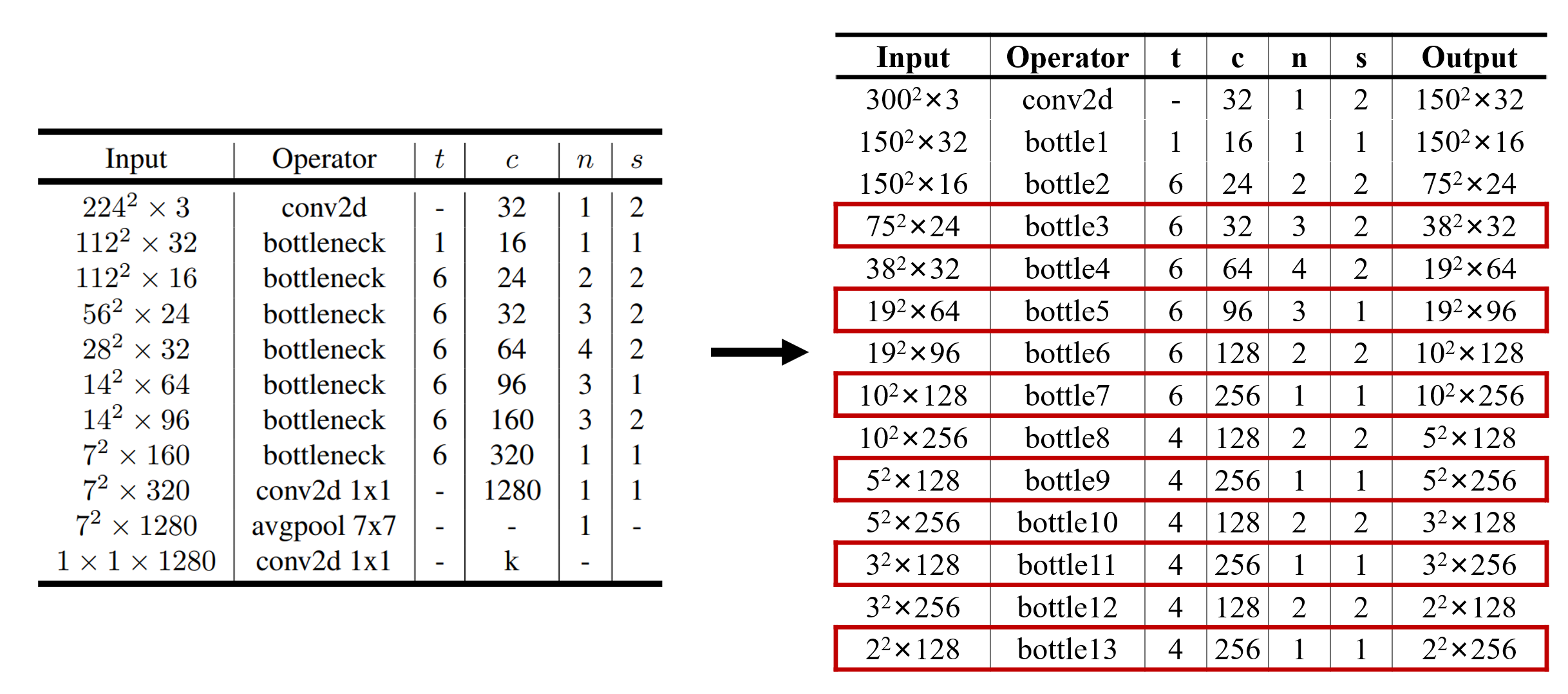
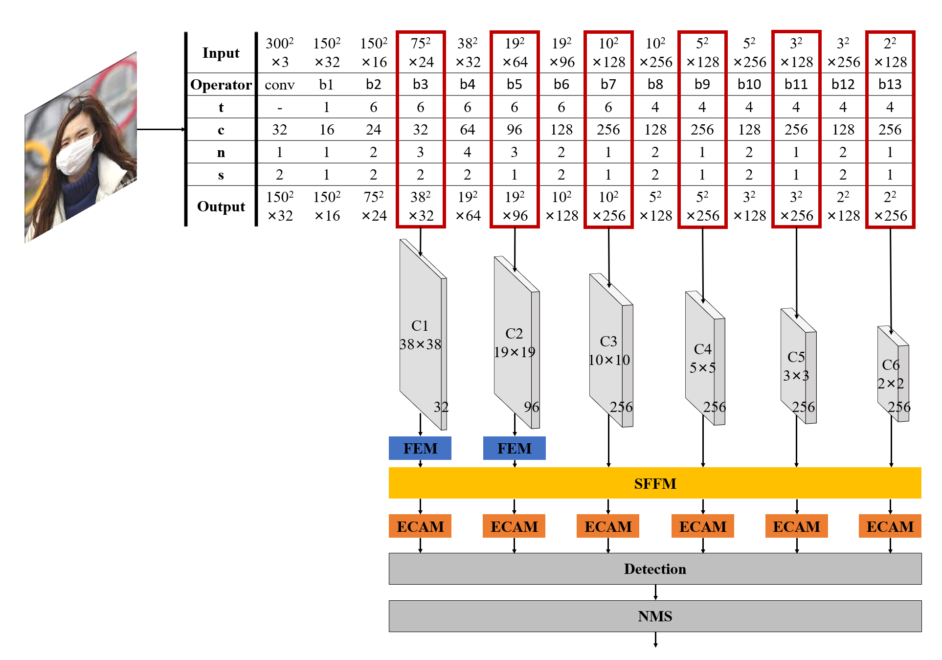
如图所示,将原主干网络vgg-16替换为MobileNetV2,保留前5个bottle层,之后以两个bottle层为基础,来进行下采样使尺度减半。具体的网络结构设计如下图所示:
即取bottle3、bottle5、bottle7、bottle9、bottle11、bottle13的输出作为特征图,特征图的尺度分别(38, 38), (19, 19), (10, 10), (5, 5), (3, 3),(2, 2)的特征图,接着对C1、C2采用FEM模块扩充通道。然后将六张特征图送入SFFM模块进行特征融合,以更好的在每张特征图上都能获取到深层与浅层信息,最后针对融合后的特征图,运用ECAM模块进行进一步的特征增强,送入Detection进行预测。
以下是网络模型代码的实现:
1 2 3 4 5 6 7 8 9 10 11 12 13 14 15 16 17 18 19 20 21 22 23 24 25 26 27 28 29 30 31 32 33 config = ((1 , 16 , 1 , 1 ),6 , 24 , 2 , 2 ),6 , 32 , 3 , 2 ),6 , 64 , 4 , 2 ),6 , 96 , 3 , 1 ),6 , 128 , 2 , 2 ),6 , 256 , 1 , 1 ),)4 , 128 , 2 , 2 ),4 , 256 , 1 , 1 ),4 , 128 , 2 , 2 ),4 , 256 , 1 , 1 ),4 , 128 , 2 , 2 ),4 , 256 , 1 , 1 ),)def get_mobilenet_v2 ():32 'conv_first' , BaseConv(3 , input_channel, stride=2 ))for i, (t, c, n, s) in enumerate (size_config):for j in range (n):if j == 0 else 1 f'bottleneck{i + 1 } _{j + 1 } ' ,f'bottle{i + 1 } ' , bottle)return layers
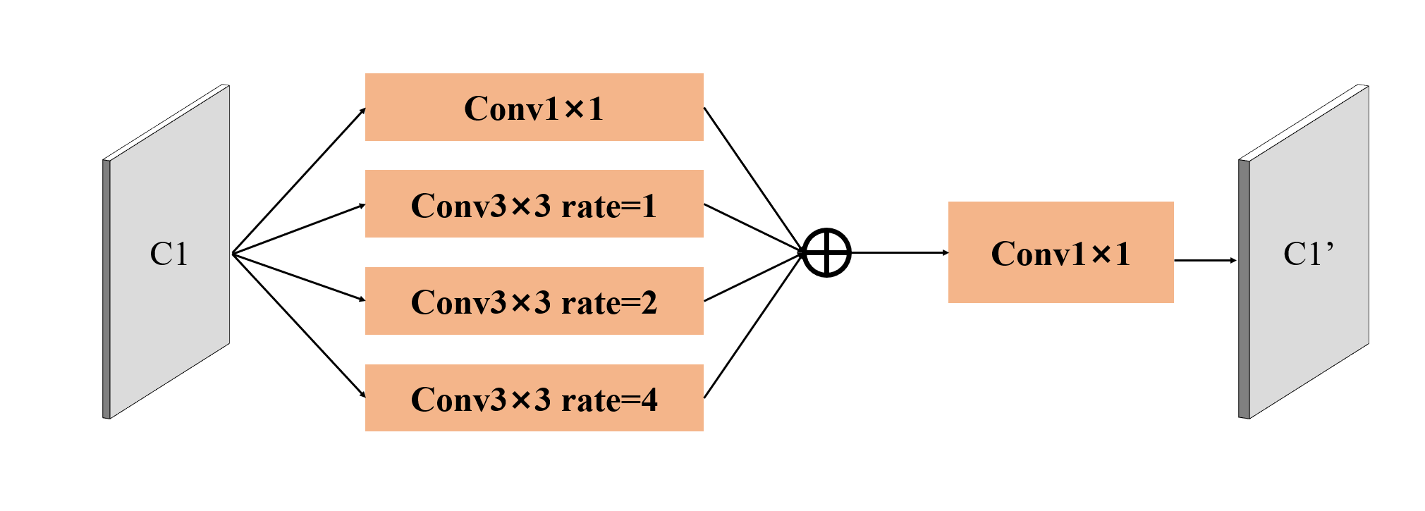
2.特征增强模块FEM(Feature Enhancement Module)
FEM模块的结构如图所示,在之前的网络结构中,可以知道C1、C2两个特征图的输出通道只有32和96,而后面的一系列的输出通道数有256,所以设计了特征增强模块。如图5所示,特征增强模块由一个卷积核大小为1×1和三个卷积核大小为3×3,通道扩张倍率分别为1、2、4的多尺度空洞卷积组成。最终将所有通道合并将特征图经过通道数不变的一个1×1的卷积以及3个通道扩张倍率分别为1、2、4的3×3卷积,最终将四个输出相加,并用通过1×1的卷积的通道数增大4倍。即C1、C2两个特征图经过FEM后分别得到通道数为128和384的特征图。具体实现如下:
1 2 3 4 5 6 7 8 9 10 11 12 13 14 15 16 17 18 class FEM (nn.Module):"""特征增强""" def __init__ (self, in_channels ):super (FEM, self).__init__()1 )3 , padding=1 , dilation=1 )3 , padding=2 , dilation=2 )3 , padding=4 , dilation=4 )4 , kernel_size=1 )def forward (self, x ):return self.cat(b1 + b2 + b3 + b4)
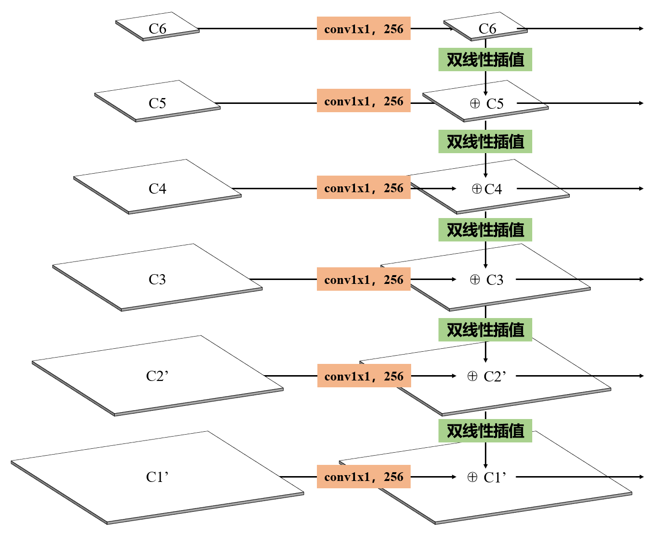
3.强特征融合模块SFFM(Strong Feature Fusion Module)
如上图所示,针对在特征图中,浅层特征图语义信息不足的问题,采用特征金字塔FPN(Feature Pyramid Network)的强特征融合策略。针对六张不同尺度的特征图,首先将每张特征图进行卷积核大小为1×1的将尺度较小的特征图经过双线性插值的方式进行上采样,然后与尺度较大的特征图相加。具体实现代码如下:
1 2 3 4 5 6 7 8 9 10 11 12 13 14 15 16 17 18 19 20 21 22 23 24 25 26 27 28 class SFFM (nn.Module):"""强特征融合""" def __init__ (self, f_map ):super (SFFM, self).__init__()256 128 , out_channels, kernel_size=1 )384 , out_channels, kernel_size=1 )256 , out_channels, kernel_size=1 )256 , out_channels, kernel_size=1 )256 , out_channels, kernel_size=1 )256 , out_channels, kernel_size=1 )4 ])3 ])2 ])1 ])0 ])def forward (self, c1, c2, c3, c4, c5, c6 ):return c1, c2, c3, c4, c5, c6
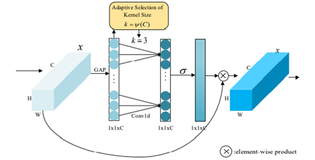
4.有效通道注意力模块ECAM(Efficient Channel Attention Module)
如图所示,ECAM模块通过全局平均池化GAP(Global Average Pooling)操作和全连接层FC(Fully Connected)来捕获特征图的每个特征通道与其k(k<9)个相邻特征通道的依赖关系,快速有效地提高对目标特征的表示。在实际过程中k取3。具体实现如下:
1 2 3 4 5 6 7 8 9 10 11 12 13 14 class ECAM (nn.Module):"""注意力模块""" def __init__ (self ):super (ECAM, self).__init__()1 )1 , 1 , kernel_size=3 , padding=1 , bias=False )def forward (self, x ):1 ).transpose(-1 , -2 )).transpose(-1 , -2 ).unsqueeze(-1 )return x * y.expand_as(x)
5.MaskSSD 将所有模块组合起来得到的模型如下:
1 2 3 4 5 6 7 8 9 10 11 12 13 14 15 16 17 18 19 20 21 22 23 24 25 26 27 28 29 30 31 32 33 34 35 36 37 38 39 40 41 42 43 44 45 46 47 48 49 50 51 52 53 54 55 56 57 58 59 60 61 62 63 64 65 66 67 68 69 70 71 72 73 74 75 76 77 78 79 80 81 82 83 84 85 86 87 88 89 90 91 92 93 94 class MaskSSD (nn.Module):""" Args: mode: train or test net: all net loc_layers: 框的位置偏置预测 conf_layers: 框的类别预测 feature_maps: 输出的特征图 num_classes: 预测的类别 + 1 confidence: 类别的置信阈值 nms_iou: 框交并比的阈值 """ def __init__ (self, mode, net, loc_layers, conf_layers, feature_maps, num_classes, confidence, nms_iou ):super (MaskSSD, self).__init__()if mode == 'test' :1 )0 , 200 , confidence, nms_iou)300 )with torch.no_grad():32 )96 )def forward (self, x ):0 ]0 ](x)1 ](tmp)2 ](tmp)3 ](tmp)4 ](c1)5 ](tmp)6 ](c2)7 ](tmp)8 ](c3)9 ](tmp)10 ](c4)11 ](tmp)12 ](c5)13 ](tmp)for (x, l, c) in zip ([c1, c2, c3, c4, c5, c6], self.loc, self.conf):0 , 2 , 3 , 1 ).flatten(start_dim=1 ))0 , 2 , 3 , 1 ).flatten(start_dim=1 ))1 ).reshape(batch_size, -1 , 4 )1 ).reshape(batch_size, -1 , self.num_classes)if self.mode == 'test' :else :return output
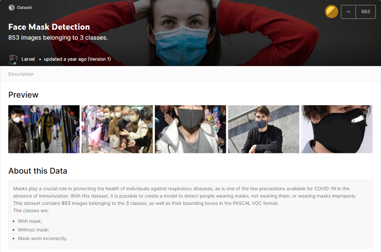
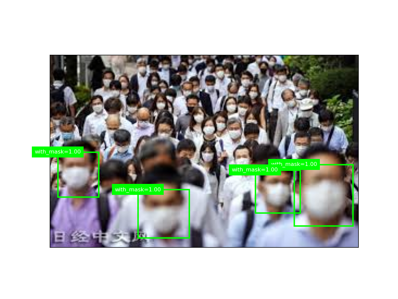
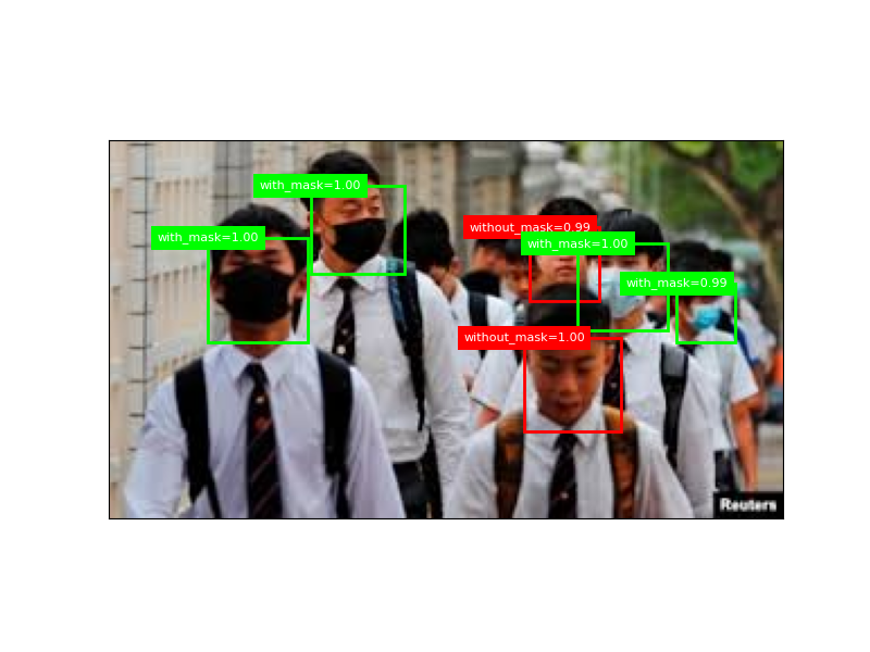
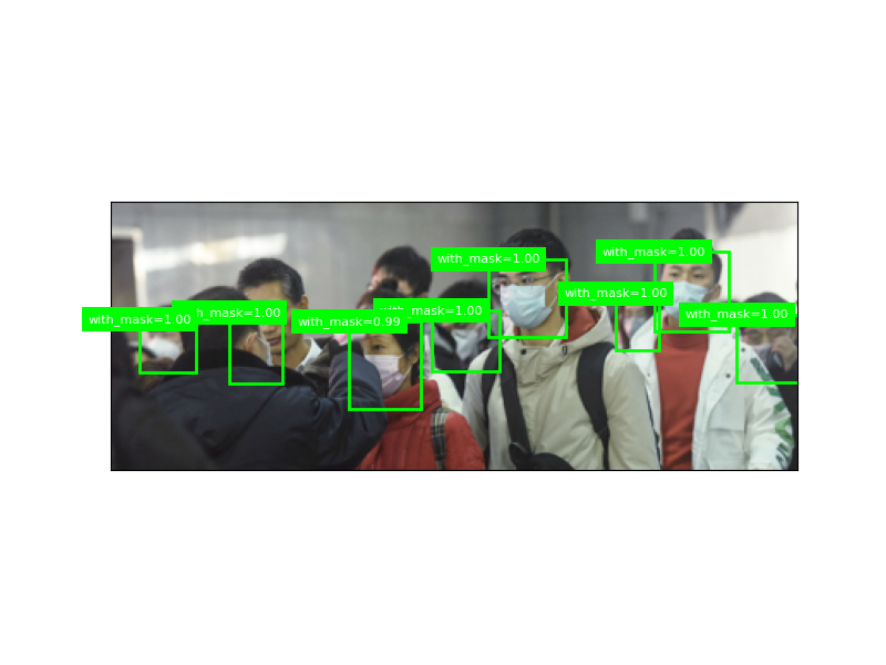
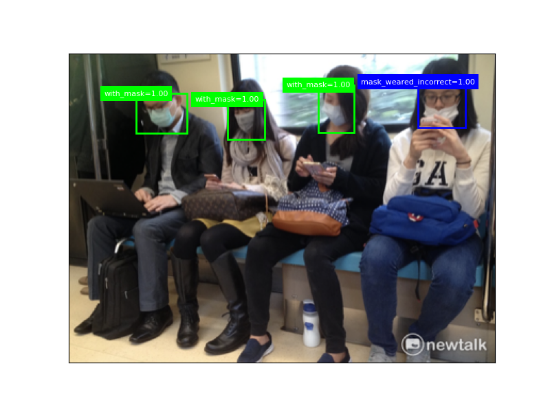
三、实例分析 1.数据集以及预处理 采用的数据集为来自Kaggle的 Face Mask Detection 数据集,其内共包含853张已标注好的数据图片共3类目标,分别为人脸已佩戴口罩、人脸未佩戴口罩以及口罩佩戴不规范。
预处理方面,将图像调整为需要输入的大小,如300×300,然后运用RGB模式下[0.485, 0.456, 0.406]的均值和[0.229, 0.224, 0.225]的标准差进行图像的归一化。对数据的读取代码如下:
1 2 3 4 5 6 7 8 9 10 11 12 13 14 15 16 17 18 19 20 21 22 23 24 25 26 27 28 29 30 31 32 33 34 35 36 37 38 39 40 41 42 43 44 45 46 47 48 49 50 51 52 53 54 55 56 57 58 def deal_target (file, p=8 ):"""对 xml 的 dic 进行处理""" with open (file) as f:'xml' )float (soup.find('height' ).text)float (soup.find('width' ).text)'object' )for ob in objects:int (ob.find('xmin' ).text) / img_wint (ob.find('ymin' ).text) / img_hint (ob.find('xmax' ).text) / img_wint (ob.find('ymax' ).text) / img_h'name' ).text'Classes' ].index(cls)])while len (boxes) < p:2 return torch.Tensor(boxes[:p])class MaskDataset (Dataset ):def __init__ (self, root, trans ):list (sorted (os.listdir(os.path.join(self.root, 'images' ))))def __getitem__ (self, idx ):'maksssksksss' + str (idx) + '.png' 'maksssksksss' + str (idx) + '.xml' 'images' , file_image)'annotations' , file_label)open (img_path).convert("RGB" )if self.trans is not None :return img, targetdef __len__ (self ):return len (self.imgs)def get_mask (path, batch_size, resize ):0.485 , 0.456 , 0.406 ], std=[0.229 , 0.224 , 0.225 ])])return data.DataLoader(trans_set, batch_size, shuffle=True , num_workers=2 ), \False , num_workers=2 )
2.运行环境和初始参数设置 在Python3.9以及Pytorch1.8的深度学习框架上进行,运行环境操作系统为Windows 10(64位),使用CUDA 11.1和进行加速GPU运算,GPU显卡为英伟达GTX 1050Ti(4G)。
模型采用均值为0,方差为0.01的正态分布进行参数的初始化设置。模型的训练采用随机梯度下降算法SGD(Stochastic Gradient Descent)对网络模型的权重参数进行更新优化,在超参数设置上,批次大小Batch Size为8,初始学习率Learning Rate为5e-3,采用动态调整方式。学习率的衰减权重Weight Decay为5e-4,动量因子Momentum取0.9,当损失函数在两轮中不再下降时,学习率调整为原来的十分之一继续训练。
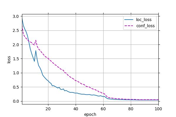
3.结果分析 模型训练的损失曲线如下图所示:
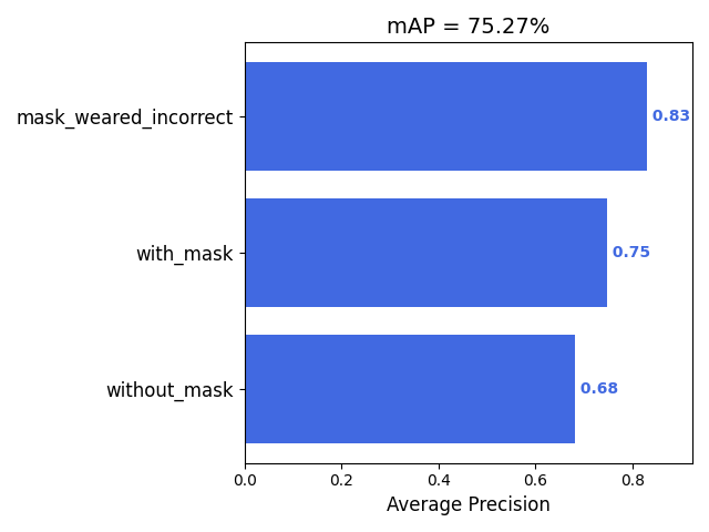
模型最终结果的mAP值如下图所示,可以发现口罩佩戴错误的识别的AP值最高
在与原SSD300的对比中,模型的参数量大大减小了,而且原SSD300不管怎么调参,损失值一直下不去,具体对比结果如图所示:
模型名称 参数大小 单epoch训练时间 识别FPS MAP Mask-SSD300 18.8M 28s 38 75.27% SSD300 92.1M
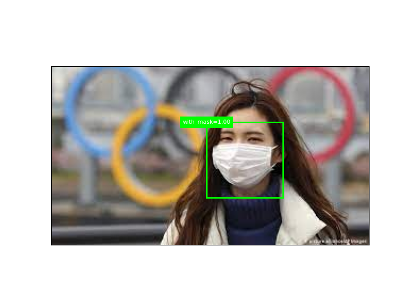
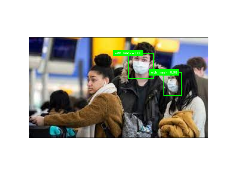
4.测试结果展示